Dental STL Model Segmentation
0. Recap
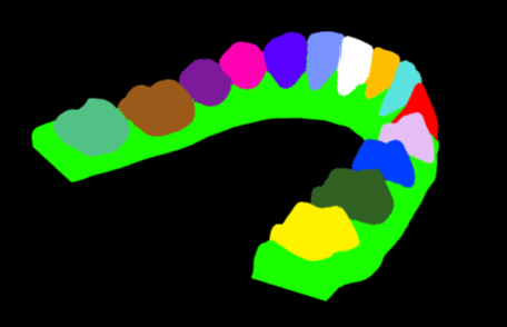
Algorithmic approach of the segmentation of a STL model (applied to dental models), and the associated optimization process.
1. Introduction
This article is drastically different from what I usually write about. But I had to work on “Dental STL Model Segmentation” for a while for work and found out about very interesting concepts, that I wanted to share here.
The code I am working on is proprietary so I can’t share it, but it’s not that hard to reproduce.
2. The Problem to solve
We are working on a program that takes a dental STL as input. But for now, it doesn’t know which part of the mesh is a tooth, and which is gum. The objective would be to preprocess the mesh to be able to precisely identify the individual tooth and the gum.
I know, it does not seem incredibly appealing when put like that (I told myself the same thing at first) BUT it’s actually quite an interesting problem, that involves the main algorithm for segmentation, but also some important and interesting optimization work (my favorite part actually, which motivated me to write this article).
3. Introduction to the Watershed algorithm
The watershed algorithm on which this work is based is a common algorithm in image processing for 2D segmentation. It uses markers placed on different zones: each marker is considered as the bottom of a basin (a minimum). All basins are filled at a constant speed, and every time two fluid-masses collision a line is drawn (the watershed).

In image processing, a topographic image is generated from the grayscaled version of the original. It’s this topographic image that is used to determine the speed at which basins fill up.
You actually don’t need to know more about this technique to understand what’s coming, but there are plenty of articles out there explaining it more in-depth. If you dive deeper into the subject, it will get a bit tricky sometimes, but I can assure you it will be worth your while if you’re into algorithmic and/or image processing.
4. Application of the Watershed algorithm to my problem
In order to achieve dental segmentation, we studied different algorithms and ways to proceed. The watershed method seemed to be the most precise one. The two main issues we will have to solve for now are :
- Applying the watershed method to this particular case, in a 3D environment
- Doing so efficiently (it should not take more than 10-15 second to complete)
Let’s only focus on the first objective for now, shall we?
I based my work on this research paper: A Fast Segmentation Method for STL Teeth Model.
It took me some time to fully understand the algorithm, but once it’s done, the implementation is quite easy because the paper contains pseudo code.
4.1. The algorithm
Here are the main steps :
-
Facet initialization
- For each face, tag it if the facet was marked by the user
-
Stack initialization
- For each tagged facet, get the three adjacent facets.
- For each neighbor, if the facet is not tagged, add it to the stack, store the curvature between the original facet and the current neighbors (I’ll come back to that) and the tooth id (the same one as the original facet).
-
Segmentation
- While the stack is not empty (while all facets are not tagged)
- Get the facet with the maximum curvature value from the stack
- Get its neighbors
- Add it to the tooth
- Remove it from the stack
- For each untagged neighbor, add it to the stack with the tooth id and the curvature
4.2. Curvature
What is the curvature, and what is used for? The curvature is comparable to the angle between two adjacent facets. Let’s consider the function H that takes two parameters, f1 the first facet and f2 the second facet. The parameter order does not matter, because :

So now the formula is the following :

with n1 being the normal direction of f1, n2 being the normal direction of f2, and the AB vector’s direction being equal to one of the non-shared sides of f2 (understand not shared between f1 and f2).

The curvature is used to sort the stack, as we always use the facet with the current highest curvature. If you remember what I told you about the Watershed algorithm, the curvatures act as the representation of the topography and are responsible for “how fast” the “liquid mass” is filling up one given pit.
5. Optimization
I am working on a web app, using typescript and ThreeJS. Javascript is far from being an efficient language. The previously presented algorithm took at first about 15min to complete on a regular-sized dental model. which is waaaaay more than requested. There are 3 main optimizations possible. The first is to code an Octree structure, the second is the use of a threshold to limit the amount of operation, and the third is to recode the algorithm in C++ and deport the calculation on the server-side.
5.1. Coding an Octree
Before talking about the Otree, you should know how a 3D object is constructed, and how the structure is referenced in ThreeJS. Every tiny triangle (face) is made of three points (vertices). Every face has three attributes (a, b, and c) that are actually pointers to a very large array, that contains the spatial positions (position vector) of every point. Sadly, if one point is shared between two faces, there are two equal position vectors in the array, at two different positions. This makes the “neighbors finding” a long a resource-consuming process.

In the example above, A and A’ are spacially equal. But their value is pointing to two different indexes in the array containing the spatial vectors. These vectors are two different objects, with the same coordinates.
It means that to check for neighbors, you have to loop through all faces and compare each vertice of the current face with the original face.
The solution to avoid all these calculations is to create a data structure, that is organized in a way, that you only loop through necessary data. Some very effective structures in spatial problems are Quadtrees (2D) or Octrees (3D). The goal is to subdivide into smaller regions recursively (depending on the number of points, or faces in our case). This creates a tree from which we will only browse necessary branches. For each facet, we try to add it to the corresponding region. If by adding the new facet, we exceed the predefined maximum for one subdivision, we subdivide it into 8 smaller regions and add the point accordingly.
In the following example, the point limit is one. It means that every time you try to add a second point to the same region, the subdivision occurs. If we were to continue the schematic, there would be a new subdivision in the region containing the red and green dots, because there can not be more than one.

The image above represents the tree aspect of an octree. The next 2 images are actual screenshots of how a dental model looks when the octree is fully drawn (the computer suffered a lot to render everything).
When zooming in, you will notice that some areas are more densely covered in cubes. These spots contain more vertices.


Now how does this speed up the neighbors finding process? Each time you want to find three neighbors, you define a cubic area around the face (of arbitrary size), and only search through regions that intersect that cube. That way, you only search for facets in specific branches, instead of looping through the entire tree.
If you want a better understanding of this data structure, I recommend this video from “Coding Train”.
PART 1 of “coding challenge: Octree” by The Coding Train
As explained earlier, the neighbors finding is a big part of the algorithm. The use of an octree allowed in this case to speed up that finding more than 10 times!
5.2. Using a threshold
The second optimization possible for this algorithm is the use of a threshold value.
If you take another look at the algorithm, we start with each tagged facet, initialize the stack, and loop until this stack is empty. Depending on the curvature, we are going to process a certain element of the stack before another. But if we admit that the start markers are placed approximatively at the center of the tooth (understand at equal distance of the two adjacents teeth), there is a certain amount of facets around the start marker that must be part of the same tooth as that starting facet.
So we determine a threshold value by testing, but it should be around 1/3 or 1/4 of the smallest distance between 2 markers.

In the example above, the green segment represents the smallest distance between 2 markers (the red dots). This allows fixing the size of each orange circle around a starting facet. Every facet contained in these circles will not be processed, and natively assigned to the tooth.
6. Conclusion
I really enjoyed working on that subject and discovered the magnificent world of optimization and data structures. I was really proud of the results I was able to get (the image used as a cover for this article is a segmented model I generated). If you have any questions, or you just want to give me your opinion about the article, I would be very happy to discuss it with you on Twitter 😉.